No… Have a think! I want you to try really! Read the chapter further - try to answer this yourself. That’s where true learning is IMO 
I’m new to this forum, can anyone give me link of colab notebook that aman was using for live streams?
Thanks
1 Like
Is last layer in simple_cnn resulted 1X1 size that means 1 pixel? this is hard to comprehend. how kernel can look at 1 pixel in last layer?
The last layer’s output is a result and the decision of it is driven by the usecase.
For example, if the use-case is to identify if something is a cat or dog, you might need one value (boolean). Anything less than 0.5 can represent cat and greater than 0.5 as Dog.
For multi class classification problems, we may get more outputs depending on the number of classes. For MNIST, we might have 10 outputs, represnting 0 to 9.
This is with regards to classification, there are other types of outputs that model can predict, like regression, boubding box and other GAN related models.
In short, dont think the resultant as neceserily an Image. It can represent anything that out use-case demands
1 Like
Hey @amanarora ,
I was reading through chapter 13 and as you mentioned in the session, I tried to visualise the convolution operation with Excel for the example that we covered of the simple_cnn network on a 28 x 28 image. Here’s how I tried to visualise it.
def conv(ni, nf, ks=3, act=True):
    res = nn.Conv2d(ni, nf, stride=2, kernel_size=ks, padding=ks//2)
    if act: res = nn.Sequential(res, nn.ReLU())
    return res

def simple_cnn():
    return sequential(
        conv(1 ,8, ks=5),    # 14 x 14
        conv(8 ,16),  # 7 x 7
        conv(16,32),  # 4 x 4
        conv(32,64),  # 2 x 2
        conv(64,10, act=False),  # 1 x 1
        Flatten(),
    )
PS: Kindly note that since a cell can only have one color, I couldn’t appropriately color all the image pixels i.e. pixels which are showing where the activation is applied are also a part of the image; basically all the cells within the padding border belong to the image; the separate coloring is just to highlight those cells because these are the positions where our convolution kernel will be applied.
In the first pass, we go from a 28 x 28 to a 14 x 14 with stride 2 and padding of 2 since kernel is bigger.

Subsequently, we get the 14 x 14 map on which we apply a smaller kernel of 3 x 3 and we get the following activation map.
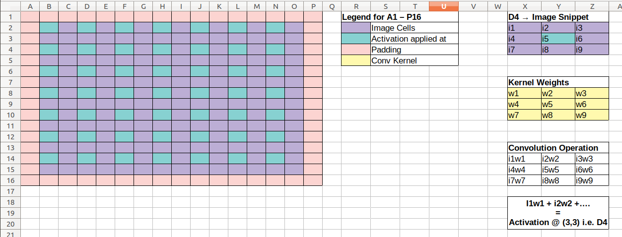
Then after applying the same kernel size a couple more times we get the following.

and then

The last map is really interesting. Here the size of the image has been reduced to 2 x 2. So, we never really see an inside pixel (as there is none). We only get to convolve over the top left corner and as a stride of 2 would throw us out of the image pixels, there’s only one convolution operation that is happening here (per kernel is implied).

I couldn’t really visualise this depthwise but I think doing this gave me a good sense of how convolutions work.
Thanks!
9 Likes
My blog post on convolution (in julia) applying various kernels:
https://nareshr8.github.io/julia-blogs/2021-08-30-convolutions.html
Let me know your comments
6 Likes
I wrote a blog post about different types of convolutions and how to use them in fastai using ConvLayer: https://ravimashru.dev/blog/2021-08-31-convolutions-in-fastai/
Would love to get some feedback
7 Likes
Thanks for talking about dilated convolutions. Do you know if dilated convolutions have anything to do with the à trous algorithm? I think they are somehow related, but haven’t quite figured out that connection at this point.
From what I’ve read, the idea of dilated convolutions did come from wavelet decomposition. That’s why they’re also called “atrous convolutions” according to A guide to convolution arithmetic for deep
learning!
2 Likes
Wow! I am so happy to see all of you progressing along nicely! This is a great feeling
1 Like
[64,4,26,26]